Bayesian Fit Indices

Introduction

Classical SEM fit indices (RMSEA, CFI, TLI, etc.) are computed from a single maximum-likelihood chi-square statistic. In Bayesian SEM, the parameters are random, so each posterior draw yields a different chi-square value and, therefore, a different set of fit indices. INLAvaan provides Bayesian analogues of the most common indices, following the framework of Garnier-Villarreal and Jorgensen (2020) (as implemented in blavaan).

This vignette covers:

1. Mathematical definitions of the Bayesian fit indices.
2. The two rescaling methods ("devM" and "MCMC").
3. A worked example with the Holzinger–Swineford data.
4. Comparison with a baseline model (incremental indices).
5. Differences between INLAvaan and blavaan.

Mathematical background

Deviance and chi-square

Let $\boldsymbol\theta^{(s)}$ denote the $s$-th posterior draw of the model parameters ($s = 1, \dots, S$). The per-sample deviance chi-square is $$\chi^2_s = 2 \bigl[\ell_{\text{sat}} - \ell(\boldsymbol\theta^{(s)})\bigr],$$ where $\ell_{\text{sat}}$ is the log-likelihood of the saturated model (sample moments equal model moments) and $\ell(\boldsymbol\theta^{(s)})$ is the log-likelihood evaluated at the $s$-th draw. This equals $N \, F_{\text{ML}}(\boldsymbol\theta^{(s)})$, where $F_{\text{ML}}$ is the ML discrepancy function.

Rescaling

INLAvaan supports two rescaling methods, controlled by the rescale argument:

"devM" (default). Uses the DIC-based effective number of parameters $p_D$. $$d_s = \chi^2_s - p_D, \qquad \mathrm{df} = p - p_D, \qquad N_{\mathrm{adj}} = N.$$ If $p_D$ is unreasonable ($p_D \leq 0$ or $p_D \geq p$), INLAvaan falls back to using $p_D = q$ (the number of free parameters).

"MCMC". Uses the classical chi-square with $N - 1$ scaling. $$d_s = \frac{N - 1}{N} \chi^2_s, \qquad \mathrm{df} = p - q, \qquad N_{\mathrm{adj}} = N - G,$$ where $q$ is the number of free parameters and $G$ is the number of groups.

In both cases the per-sample noncentrality parameter is $\hat\lambda_s = \max(d_s - \mathrm{df},\, 0)$.

Absolute fit indices

The following indices are computed at each posterior draw $s$, generating a posterior distribution.

BRMSEA (Bayesian RMSEA). $$\text{BRMSEA}_s = \sqrt{\frac{\hat\lambda_s}{\mathrm{df} \cdot N_\text{adj}}} \cdot \sqrt{G}.$$

BGammaHat. $$\text{BGammaHat}_s = \frac{v}{v + 2\hat\lambda_s / N_\text{adj}},$$ where $v = \sum_g p_g$ is the total number of observed variables across groups.

Adjusted BGammaHat. $$\text{adjBGammaHat}_s = 1 - \frac{p}{\mathrm{df}} \bigl(1 - \text{BGammaHat}_s\bigr).$$

BMc (McDonald’s centrality index). $$\text{BMc}_s = \exp\!\bigl(-\tfrac{1}{2}\hat\lambda_s / N_\text{adj}\bigr).$$

Incremental fit indices

Incremental indices compare the target model against a baseline (null) model. Let $d_s^{(0)}$, $\mathrm{df}^{(0)}$, and $\hat\lambda_s^{(0)}$ denote the corresponding quantities for the baseline model.

BCFI (Bayesian CFI). $$\text{BCFI}_s = 1 - \frac{\hat\lambda_s}{\hat\lambda_s^{(0)}}.$$

BTLI (Bayesian TLI). $$\text{BTLI}_s = \frac{d_s^{(0)} / \mathrm{df}^{(0)} - d_s / \mathrm{df}}{d_s^{(0)} / \mathrm{df}^{(0)} - 1}.$$

BNFI (Bayesian NFI). $$\text{BNFI}_s = \frac{d_s^{(0)} - d_s}{d_s^{(0)}}.$$

The posterior expectations (EAP), standard deviations, quantile-based credible intervals, and modes of these distributions are reported by the summary() method.

Example: three-factor CFA

We fit a three-factor CFA on the Holzinger–Swineford (1939) data.

HS.model <- "
  visual  =~ x1 + x2 + x3
  textual =~ x4 + x5 + x6
  speed   =~ x7 + x8 + x9
"

fit <- acfa(HS.model, HolzingerSwineford1939, verbose = FALSE)

Scalar fit measures

fitMeasures() returns the posterior mean (EAP) of each Bayesian fit index alongside the marginal log-likelihood, ppp, DIC, and gradient diagnostics.

fitMeasures(fit)
#>         npar   margloglik          ppp          dic        p_dic       BRMSEA 
#>           21    -3823.429        0.000     7516.853       20.461        0.091 
#>    BGammaHat adjBGammaHat          BMc 
#>        0.957        0.921        0.904

Posterior distributions of fit indices

To inspect the full posterior distribution of each index, use bfit_indices(). This returns an S3 object of class "bfit_indices".

bfi <- bfit_indices(fit)
bfi
#> Posterior summary of devM-based Bayesian fit indices (nsamp = 1000): 
#> 
#>       BRMSEA    BGammaHat adjBGammaHat          BMc 
#>        0.091        0.957        0.920        0.903

Calling summary() provides a table of posterior summaries (Mean, SD, 2.5%, 50%, 97.5%, Mode) for each index.

summary(bfi)
#> 
#> Posterior summary of devM-based Bayesian fit indices (nsamp = 1000):
#> 
#>               Mean    SD X2.5.  X25.  X50.  X75. X97.5.  Mode
#> BRMSEA       0.091 0.005 0.083 0.087 0.091 0.094  0.102 0.090
#> BGammaHat    0.957 0.005 0.946 0.954 0.957 0.960  0.964 0.958
#> adjBGammaHat 0.920 0.008 0.901 0.915 0.921 0.927  0.934 0.924
#> BMc          0.903 0.010 0.879 0.897 0.904 0.910  0.920 0.907

You can also access the raw per-sample vectors for custom analysis:

hist(bfi$indices$BRMSEA, breaks = 30, main = "BRMSEA", xlab = "BRMSEA",
     col = "steelblue", border = "white")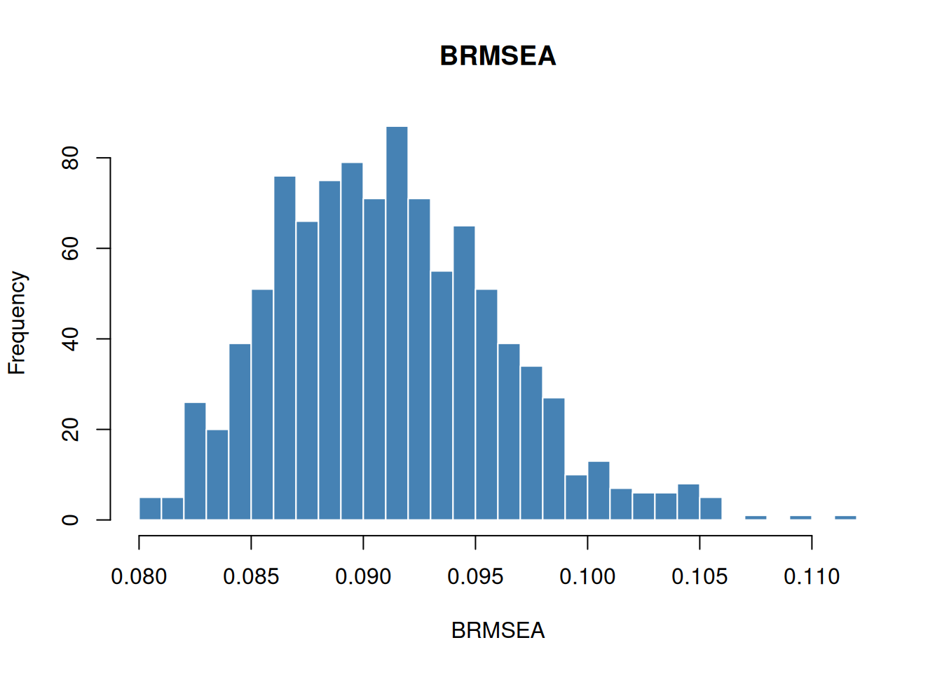

Posterior distribution of BRMSEA

Comparison with a baseline model

Incremental indices (BCFI, BTLI, BNFI) require a baseline model. A common choice is the independence (uncorrelated) model.

null.model <- "
  x1 ~~ x1
  x2 ~~ x2
  x3 ~~ x3
  x4 ~~ x4
  x5 ~~ x5
  x6 ~~ x6
  x7 ~~ x7
  x8 ~~ x8
  x9 ~~ x9
"

fit_null <- acfa(null.model, HolzingerSwineford1939, verbose = FALSE)

Now pass the baseline model to fitMeasures() or bfit_indices():

fitMeasures(fit, baseline.model = fit_null)
#>         npar   margloglik          ppp          dic        p_dic       BRMSEA 
#>           21    -3823.429        0.000     7516.853       20.461        0.091 
#>    BGammaHat adjBGammaHat          BMc         BCFI         BTLI         BNFI 
#>        0.957        0.921        0.903        0.931        0.898        0.907

bfi_inc <- bfit_indices(fit, baseline.model = fit_null)
summary(bfi_inc)
#> 
#> Posterior summary of devM-based Bayesian fit indices (nsamp = 1000):
#> 
#>               Mean    SD X2.5.  X25.  X50.  X75. X97.5.  Mode
#> BRMSEA       0.091 0.005 0.083 0.088 0.091 0.094  0.102 0.089
#> BGammaHat    0.956 0.005 0.946 0.954 0.957 0.960  0.964 0.958
#> adjBGammaHat 0.920 0.008 0.902 0.915 0.921 0.926  0.934 0.924
#> BMc          0.903 0.010 0.881 0.897 0.904 0.910  0.919 0.907
#> BCFI         0.930 0.008 0.913 0.926 0.931 0.935  0.942 0.933
#> BTLI         0.897 0.011 0.872 0.891 0.898 0.905  0.915 0.902
#> BNFI         0.906 0.007 0.890 0.902 0.907 0.911  0.918 0.909

Rescaling: "devM" vs "MCMC"

The rescale argument controls how the chi-square and degrees of freedom are computed. The default is "devM", which subtracts the DIC-based $p_D$ from the deviance. To use the classical $N - 1$ scaling instead, set rescale = "MCMC":

bfi_mcmc <- bfit_indices(fit, rescale = "MCMC")
summary(bfi_mcmc)
#> 
#> Posterior summary of MCMC-based Bayesian fit indices (nsamp = 1000):
#> 
#>               Mean    SD X2.5.  X25.  X50.  X75. X97.5.  Mode
#> BRMSEA       0.107 0.004 0.099 0.104 0.107 0.110  0.117 0.105
#> BGammaHat    0.943 0.005 0.932 0.940 0.943 0.946  0.950 0.945
#> adjBGammaHat 0.892 0.009 0.873 0.887 0.893 0.898  0.906 0.896
#> BMc          0.872 0.010 0.849 0.866 0.873 0.879  0.888 0.876

The two methods will generally produce different results, especially with informative priors or when $p_D$ deviates substantially from $q$.

Differences from blavaan

INLAvaan’s Bayesian fit indices follow the same mathematical framework as blavaan (Merkle et al. 2021), with a few implementation differences:

Feature	INLAvaan	blavaan
Posterior samples	INLA-based (Sobol/NORTA)	MCMC draws from Stan/JAGS
Rescaling methods	"devM", "MCMC"	"devM", "MCMC", "ppmc"
Effective parameters ($p_D$)	DIC-based $p_D$ only	DIC-based $p_D$, LOOIC-based $p_{\text{loo}}$, or WAIC-based $p_{\text{waic}}$
HPD intervals	Not currently computed	Computed via {coda}
Summary statistics	Mean, SD, 2.5%, 50%, 97.5%, Mode	EAP, Median, MAP, SD, HPD
Return class	S3 "bfit_indices"	S4 "blavFitIndices"

Currently, INLAvaan only supports $p_D$ from the DIC (i.e., p_dic). The "ppmc" rescaling method (which computes replicated data under the posterior predictive) is not yet available.

References

Garnier-Villarreal, Mauricio, and Terrence D. Jorgensen. 2020. “Bayesian Structural Equation Modeling with Cross-Loadings and Residual Covariances: Comments on Asparouhov and Muthén.” Journal of Educational and Behavioral Statistics 45 (2): 198–223. https://doi.org/10.3102/1076998619877529.

Merkle, Edgar C., Ellen Fitzsimmons, James Uanhoro, and Ben Goodrich. 2021. “Blavaan: Bayesian Structural Equation Models via Parameter Expansion.” Journal of Statistical Software 100 (6): 1–33. https://doi.org/10.18637/jss.v100.i06.