Get started

Introduction

SEMs are ubiquitous in the social sciences, psychology, ecology, and other fields. The INLAvaan package provides a user-friendly interface for fitting Bayesian SEMs using Integrated Nested Laplace Approximations (INLA, Rue, Martino, and Chopin 2009). This vignette will guide you through the basics of using INLAvaan to fit a simple SEM. Before we begin make sure you have installed the INLAvaan package from GitHub by running the commands below.

# Run this if you have not yet installed INLAvaan
install.packages("pak")
pak::pak("haziqj/INLAvaan")

# Load all libraries for this example
library(INLAvaan)
library(tidyverse)
library(lavaan)

Motivating example

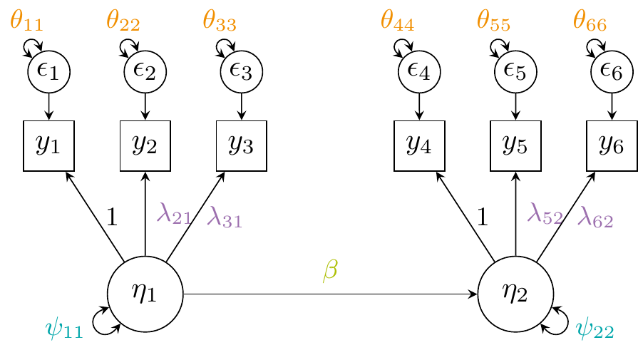
To motivate the use of SEMs, consider the introductory example in Song and Lee (2012): Does poorer glycemic control lead to greater severity of kidney disease? We observe three indicators of glycemic control ($y_1$, $y_2$, $y_3$) and three indicators of kidney disease severity ($y_4$, $y_5$, $y_6$).

Rather than fitting separate regression models for each indicator, SEM allows us to model the relationship between the latent constructs themselves, providing a clearer and more coherent representation of the underlying processes. The hypothesised SEM is illustrated by the figure below:

Data

For the two-factor SEM we described above, it is easy to simulate some data using the lavaan package to do so. The code is below:

pop_mod <- "
  eta1 =~ 1*y1 + 0.8*y2 + 0.6*y3
  eta2 =~ 1*y4 + 0.8*y5 + 0.6*y6
  eta2 ~ 0.3*eta1
  
  # Variances
  y1 ~~ 0.5*y1
  y2 ~~ 0.5*y2
  y3 ~~ 0.5*y3
  y4 ~~ 0.5*y4
  y5 ~~ 0.5*y5
  y6 ~~ 0.5*y6
  eta1 ~~ 1*eta1
  eta2 ~~ 1*eta2
"
set.seed(123)
dat <- lavaan::simulateData(pop_mod, sample.nobs = 1000)
glimpse(dat)
#> Rows: 1,000
#> Columns: 6
#> $ y1 <dbl> 1.1455803, 1.4947024, -1.2456403, -0.1086872, 1.0923138, -1.2380598…
#> $ y2 <dbl> 0.91137657, 0.72401293, -1.25960940, 0.76466115, 2.19814346, -2.548…
#> $ y3 <dbl> 0.921500064, -0.207810400, -0.485685595, -0.699851026, 1.305249049,…
#> $ y4 <dbl> -0.14207811, -0.37935984, -0.96230121, 0.38055295, -2.82223505, -1.…
#> $ y5 <dbl> 0.22887213, -0.49975381, -0.94007870, -1.22195516, -1.55233455, -0.…
#> $ y6 <dbl> -0.43559523, -0.21900233, -2.15905213, 0.48356421, 0.83857184, -1.0…

From the code above, note the true values of the parameters, including the factor loadings $\Lambda$, regression coefficient $\beta$ between the two latent variables, as well as the residual and latent variances $\Theta$ and $\Psi$ respectively.

Model fit

Now that we have simulated some data, we can fit the SEM using INLAvaan. The model syntax is similar to that of lavaan, making it easy to specify the model. For further details on the model syntax, refer to the lavaan website. INLAvaan provides mirror functions for the main model fitting functions in lavaan:

• acfa() mirrors lavaan::cfa() for confirmatory factor analysis; and
• asem() mirrors lavaan::sem() for structural equation models;
• agrowth() mirrors lavaan::growth() for latent growth curve models.

The code to fit the SEM model is below:

mod <- "
  eta1 =~ y1 + y2 + y3
  eta2 =~ y4 + y5 + y6
  eta2 ~ eta1
"
fit <- asem(mod, dat)
#> ℹ Using MVN log-likelihood.
#> ℹ Finding posterior mode.
#> ✔ Finding posterior mode. [113ms]
#> 
#> ℹ Computing the Hessian.
#> ✔ Computing the Hessian. [181ms]
#> 
#> ℹ Performing VB correction.
#> ✔ Performing VB correction. [217ms]
#> 
#> ℹ Using skew normal approximation.
#> ⠙ Fitting skew normal to 0/13 marginals.
#> ✔ Fitting skew normal to 13/13 marginals. [632ms]
#> 
#> ⠙ Computing ppp and DIC.
#> ⠹ Computing ppp and DIC.
#> ✔ Computing ppp and DIC. [1.5s]
#> 

INLAvaan computes an approximation to the posterior density by way of a Laplace approximation (Tierney, Kass, and Kadane 1989). The joint mode and the Hessian needs to be computed, which gives a Gaussian distribution for the joint posterior of the parameters. The default method for optimisation is stats::nlminb(), but other optimisers can be used by specifying optim_method = "ucminf" for the ucminf package or optim_method = "optim" to call the stats::optim() function with method "BFGS".

From this, marginal posterior distributions for each parameter can be obtained by one of several ways, including 1) Skew normal fitting (marginal_method = "skewnorm", the default method, see Chiuchiolo, Van Niekerk, and Rue 2023); 2) Two-piece asymmetric Gaussian fitting (marginal_method = "asymgaus", see Martins et al. 2013); 3) Direct marginalisation of the joint Gaussian posterior (marginal_method = "marggaus"); and 4) Sampling from the joint Gaussian posterior (marginal_method = "sampling").

Once the marginal posterior distributions have been obtained, we can further use these to compute any derived quantities of interest via copula sampling. The posterior predictive p-values (Gelman, Meng, and Stern 1996) and Deviance Information Criterion (DIC, Spiegelhalter et al. 2002) are computed this way. Often, the posterior sampling takes longer than the model fitting itself, so the number of samples can be controlled via the nsamp argument (default is nsamp = 1000) or can be skipped altoghether (test = "none").

Methods

The resulting object is of class INLAvaan, a subclass of lavaan objects.

str(fit, 1)
#> Formal class 'INLAvaan' [package "INLAvaan"] with 21 slots
fit
#> INLAvaan 0.2.0.9004 ended normally after 62 iterations
#> 
#>   Estimator                                      BAYES
#>   Optimization method                           NLMINB
#>   Number of model parameters                        13
#> 
#>   Number of observations                          1000
#> 
#> Model Test (User Model):
#> 
#>    Marginal log-likelihood                   -8069.067 
#>    PPP (Chi-square)                              0.327

As a result, most of the methods that work for lavaan objects will also work for INLAvaan objects. The most common ones are probably coef() and summary().

# Inspect coefficients
coef(fit)
#>   eta1=~y2   eta1=~y3   eta2=~y5   eta2=~y6  eta2~eta1     y1~~y1     y2~~y2 
#>      0.873      0.602      0.786      0.582      0.272      0.487      0.499 
#>     y3~~y3     y4~~y4     y5~~y5     y6~~y6 eta1~~eta1 eta2~~eta2 
#>      0.489      0.476      0.464      0.522      1.050      0.931

# Summary of results
summary(fit)
#> INLAvaan 0.2.0.9004 ended normally after 62 iterations
#> 
#>   Estimator                                      BAYES
#>   Optimization method                           NLMINB
#>   Number of model parameters                        13
#> 
#>   Number of observations                          1000
#> 
#> Model Test (User Model):
#> 
#>    Marginal log-likelihood                   -8069.067 
#>    PPP (Chi-square)                              0.327 
#> 
#> Information Criteria:
#> 
#>    Deviance (DIC)                            16031.240 
#>    Effective parameters (pD)                    12.698 
#> 
#> Parameter Estimates:
#> 
#>    Marginalisation method                     SKEWNORM
#>    VB correction                                  TRUE
#> 
#> Latent Variables:
#>                    Estimate       SD     2.5%    97.5%      KLD    Prior       
#>   eta1 =~                                                                      
#>     y1                1.000                                                    
#>     y2                0.873    0.043    0.791    0.960    0.007    normal(0,10)
#>     y3                0.602    0.032    0.540    0.665    0.003    normal(0,10)
#>   eta2 =~                                                                      
#>     y4                1.000                                                    
#>     y5                0.786    0.042    0.706    0.871    0.002    normal(0,10)
#>     y6                0.582    0.034    0.516    0.650    0.001    normal(0,10)
#> 
#> Regressions:
#>                    Estimate       SD     2.5%    97.5%      KLD    Prior       
#>   eta2 ~                                                                       
#>     eta1              0.272    0.038    0.197    0.347    0.000    normal(0,10)
#> 
#> Variances:
#>                    Estimate       SD     2.5%    97.5%      KLD    Prior       
#>    .y1                0.487    0.047    0.400    0.585    0.000 gamma(1,.5)[sd]
#>    .y2                0.499    0.039    0.427    0.579    0.001 gamma(1,.5)[sd]
#>    .y3                0.489    0.027    0.438    0.544    0.003 gamma(1,.5)[sd]
#>    .y4                0.476    0.050    0.383    0.579    0.001 gamma(1,.5)[sd]
#>    .y5                0.464    0.035    0.400    0.536    0.000 gamma(1,.5)[sd]
#>    .y6                0.522    0.028    0.469    0.580    0.004 gamma(1,.5)[sd]
#>     eta1              1.050    0.077    0.907    1.210    0.005 gamma(1,.5)[sd]
#>    .eta2              0.931    0.073    0.796    1.082    0.001 gamma(1,.5)[sd]

It’s possible to request posterior medians and modes in the summary output by specifying postmedian = TRUE or postmode = TRUE in the summary() function.

Predictions

Predicted values for the latent variables can be obtained using the predict() function. This is done by sampling from the posterior distributions of the latent variables given the observed data. In the future, this function will also allow for out-of-sample predictions and also to retrieve predictions for observed variables.

eta_preds <- predict(fit, nsamp = 100)
#> Sampling latent variables ■■■                                8% | ETA: 18s
#> Sampling latent variables ■■■■■■■■                          23% | ETA: 15s
#> Sampling latent variables ■■■■■■■■■■■■■                     39% | ETA: 12s
#> Sampling latent variables ■■■■■■■■■■■■■■■■■                 55% | ETA:  9s
#> Sampling latent variables ■■■■■■■■■■■■■■■■■■■■■■            70% | ETA:  6s
#> Sampling latent variables ■■■■■■■■■■■■■■■■■■■■■■■■■■■       85% | ETA:  3s
#> Sampling latent variables ■■■■■■■■■■■■■■■■■■■■■■■■■■■■■■■  100% | ETA:  0s
#> 
length(eta_preds)
#> [1] 100
head(eta_preds[[1]])
#>             eta1       eta2
#> [1,]  1.37852006  0.3137931
#> [2,] -0.05476344  0.1054589
#> [3,] -1.21496420 -1.4148097
#> [4,]  0.31214603 -0.5080118
#> [5,]  1.00553115 -1.8027183
#> [6,] -1.79279552 -1.3659592

This is an S3 object with a summary method that provides posterior means and credible intervals for the latent variables. Alternatively, the user is welcome to perform their own summary statistics on the list of posterior samples returned by predict().

summ_eta <- summary(eta_preds)
str(summ_eta)
#> List of 6
#>  $ group_id: NULL
#>  $ Mean    : num [1:1000, 1:2] 0.9966 0.7301 -1.1596 0.0778 1.2994 ...
#>   ..- attr(*, "dimnames")=List of 2
#>   .. ..$ : NULL
#>   .. ..$ : chr [1:2] "eta1" "eta2"
#>  $ SD      : num [1:1000, 1:2] 0.456 0.412 0.461 0.42 0.43 ...
#>   ..- attr(*, "dimnames")=List of 2
#>   .. ..$ : NULL
#>   .. ..$ : chr [1:2] "eta1" "eta2"
#>  $ 2.5%    : num [1:1000, 1:2] 0.1412 -0.0508 -1.9647 -0.6443 0.4714 ...
#>   ..- attr(*, "dimnames")=List of 2
#>   .. ..$ : NULL
#>   .. ..$ : chr [1:2] "eta1" "eta2"
#>  $ 50%     : num [1:1000, 1:2] 1.0262 0.7335 -1.1692 0.0709 1.3152 ...
#>   ..- attr(*, "dimnames")=List of 2
#>   .. ..$ : NULL
#>   .. ..$ : chr [1:2] "eta1" "eta2"
#>  $ 97.5%   : num [1:1000, 1:2] 1.875 1.597 -0.433 0.811 2.097 ...
#>   ..- attr(*, "dimnames")=List of 2
#>   .. ..$ : NULL
#>   .. ..$ : chr [1:2] "eta1" "eta2"
#>  - attr(*, "class")= chr "summary.predict.inlavaan_internal"
head(summ_eta$Mean)
#>             eta1        eta2
#> [1,]  0.99659688 -0.01089038
#> [2,]  0.73008173 -0.25780032
#> [3,] -1.15963614 -1.26547645
#> [4,]  0.07776609 -0.24572359
#> [5,]  1.29938160 -1.37475344
#> [6,] -1.74244781 -0.88130558

Plot

A simple plot method is provided to view the marginal posterior distributions of the parameters. The vertical lines indicate the posterior mode.

plot(fit)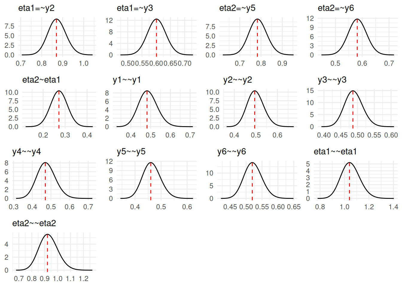

Model comparison

In addition to several global fit indices (i.e. PPP, DIC), it is possible to compare models by way of Bayes factors using the compare() function. This function takes two INLAvaan objects and computes the Bayes factor using the Laplace approximations to the marginal likelihoods.

mod2 <- "
  # A model with uncorrelated factors
  eta1 =~ y1 + y2 + y3
  eta2 =~ y4 + y5 + y6
  eta1 ~~ 0*eta2
"
fit2 <- asem(mod2, dat)
#> ℹ Using MVN log-likelihood.
#> ℹ Finding posterior mode.
#> ✔ Finding posterior mode. [125ms]
#> 
#> ℹ Computing the Hessian.
#> ✔ Computing the Hessian. [152ms]
#> 
#> ℹ Performing VB correction.
#> ✔ Performing VB correction. [218ms]
#> 
#> ℹ Using skew normal approximation.
#> ⠙ Fitting skew normal to 0/12 marginals.
#> ✔ Fitting skew normal to 12/12 marginals. [600ms]
#> 
#> ⠙ Computing ppp and DIC.
#> ✔ Computing ppp and DIC. [1.4s]
#> 
compare(fit, fit2)
#> Bayesian Model Comparison (INLAvaan)
#> Models ordered by marginal log-likelihood
#> 
#>  Model No.params Marg.Loglik      DIC       pD   logBF
#>    fit        13   -8069.067 16031.24 12.69765   0.000
#>   fit2        12   -8088.871 16082.69 12.35877 -19.804

As a note, there have been several criticisms of the use of Bayes factors for model comparison, particularly in the context of SEMs (Tendeiro and Kiers 2019; Schad et al. 2023). The blavaan package is able to implement WAICs and LOOs as alternative model comparison metrics, and these will hopefully also be implemented in future versions of INLAvaan.

Setting priors

The INLAvaan package uses the same prior specification syntax as blavaan (Merkle and Rosseel 2018; Merkle et al. 2021), as detailed here. Essentially, there are two ways to set priors for model parameters: 1) Globally for all parameters of a certain type (e.g., all factor loadings, all regression coefficients, etc.); and 2) Individually for specific parameters in the model syntax.

The default global priors are derived from blavaan:

blavaan::dpriors()
#>                nu             alpha            lambda              beta 
#>    "normal(0,32)"    "normal(0,10)"    "normal(0,10)"    "normal(0,10)" 
#>             theta               psi               rho             ibpsi 
#> "gamma(1,.5)[sd]" "gamma(1,.5)[sd]"       "beta(1,1)" "wishart(3,iden)" 
#>               tau 
#>   "normal(0,1.5)"

Note that, INLAvaan uses the SRS decomposition on variance matrices, and consequently places priors on correlations instead of covariances. If, instead we wished to set global priors, say a Gamma distribution on variances instead of standard deviations (default), then we would do the following:

DP <- blavaan::dpriors(theta = "gamma(1,1)", psi = "gamma(1,1)")
DP
#>                nu             alpha            lambda              beta 
#>    "normal(0,32)"    "normal(0,10)"    "normal(0,10)"    "normal(0,10)" 
#>             theta               psi               rho             ibpsi 
#>      "gamma(1,1)"      "gamma(1,1)"       "beta(1,1)" "wishart(3,iden)" 
#>               tau 
#>   "normal(0,1.5)"
## fit <- asem(mod, dat, dpriors = DP)  # not run

To set individual priors for specific parameters, we can do so in the model syntax itself. For instance, to set a normal prior with mean 1 and standard deviation 3 for the factor loading of y3 on eta1, and a normal prior with mean 0 and standard deviation 0.5 for the regression coefficient from eta1 to eta2, we would specify the model as follows:

mod <- "
  eta1 =~ y1 + y2 + prior('normal(1,3)')*y3
  eta2 =~ y4 + y5 + y6
  eta2 ~ prior('normal(0,.5)')*eta1
"
## fit <- asem(mod, dat)  # not run

Dependency on R-INLA

Dependency on R-INLA has been temporarily removed for tThe current version of INLAvaan (v0.2-0). For a wide class LVMs and SEMs where the latent variables are unstructured and independent, the current implementation is sufficient. However, future versions of INLAvaan will re-introduce dependency on R-INLA to allow for more complex latent structures, such as spatial and temporal dependencies.

References

Chiuchiolo, Cristian, Janet Van Niekerk, and Håvard Rue. 2023. “Joint Posterior Inference for Latent Gaussian Models with R-INLA.” Journal of Statistical Computation and Simulation 93 (5): 723–52. https://doi.org/10.1080/00949655.2022.2117813.

Gelman, Andrew, Xiao-Li Meng, and Hal Stern. 1996. “Posterior Predictive Assessment of Model Fitness Via Realized Discrepancies.” Statistica Sinica 6 (4): 733–60. https://www.jstor.org/stable/24306036.

Martins, Thiago G., Daniel Simpson, Finn Lindgren, and Håvard Rue. 2013. “Bayesian Computing with INLA: New Features.” Computational Statistics & Data Analysis 67 (November): 68–83. https://doi.org/10.1016/j.csda.2013.04.014.

Merkle, Edgar C., Ellen Fitzsimmons, James Uanhoro, and Ben Goodrich. 2021. “Efficient Bayesian Structural Equation Modeling in Stan.” Journal of Statistical Software 100 (November): 1–22. https://doi.org/10.18637/jss.v100.i06.

Merkle, Edgar C., and Yves Rosseel. 2018. “blavaan: Bayesian Structural Equation Models via Parameter Expansion.” Journal of Statistical Software 85 (June): 1–30. https://doi.org/10.18637/jss.v085.i04.

Rue, Håvard, Sara Martino, and Nicolas Chopin. 2009. “Approximate Bayesian Inference for Latent Gaussian Models by Using Integrated Nested Laplace Approximations.” Journal of the Royal Statistical Society Series B: Statistical Methodology 71 (2): 319–92. https://doi.org/10.1111/j.1467-9868.2008.00700.x.

Schad, Daniel J., Bruno Nicenboim, Paul-Christian Bürkner, Michael Betancourt, and Shravan Vasishth. 2023. “Workflow Techniques for the Robust Use of Bayes Factors.” Psychological Methods 28 (6): 1404–26. https://doi.org/10.1037/met0000472.

Song, Xin‐Yuan, and Sik‐Yum Lee. 2012. Basic and Advanced Bayesian Structural Equation Modeling: With Applications in the Medical and Behavioral Sciences. 1st ed. Wiley Series in Probability and Statistics. Wiley. https://doi.org/10.1002/9781118358887.

Spiegelhalter, David J, Nicola G Best, Bradley P Carlin, and Angelika Van Der Linde. 2002. “Bayesian Measures of Model Complexity and Fit.” Journal of the Royal Statistical Society Series B: Statistical Methodology 64 (4): 583–639.

Tendeiro, Jorge N., and Henk A. L. Kiers. 2019. “A Review of Issues about Null Hypothesis Bayesian Testing.” Psychological Methods 24 (6): 774–95. https://doi.org/10.1037/met0000221.

Tierney, Luke, Robert E. Kass, and Joseph B. Kadane. 1989. “Fully Exponential Laplace Approximations to Expectations and Variances of Nonpositive Functions.” Journal of the American Statistical Association 84 (407): 710–16. https://doi.org/10.1080/01621459.1989.10478824.