Binary CFA

As of version 0.2.1.9000, INLAvaan supports the fitting of binary data for CFA using the pairwise likelihood function available from lavaan. This is an experimental feature which needs further research and testing. Some notes:

• Using PML is considered a “limited-information” approach, due to pairwise likelihood contributions not utilising the fully joint information in the data.
• The scale of the PML function will significantly be different, since the total pairwise log-likelihood adds up contributions in pairs. Following the literature on spatial models using composite likelihoods, INLAvaan adjusts this by a factor of $1/\sqrt{p}$.
• It is proabably unwise to use the Laplace-approximated marginal likelihood for model comparison. The ppp also may not be suitable for ordinal data and needs a rethink.
• Bayesian estimation of CFA favours the parameterization = "theta" option, since the priors on residual variances are more intuitive to specify. INLAvaan switches to this by default.
• For binary models, normal priors for the thresholds should be fine. But looking ahead for ordinal models, the priors for thresholds should be specified in such a way that the ordering is preserved $\tau_0 < \tau_1 < \tau_2 < \cdots < \tau_k$. This is not yet implemented in INLAvaan.

Having said that, let’s take a look at how binary CFA can be implemented in INLAvaan.

library(INLAvaan)
library(blavaan)
#> Loading required package: Rcpp
#> This is blavaan 0.5-10
#> On multicore systems, we suggest use of future::plan("multicore") or
#>   future::plan("multisession") for faster post-MCMC computations.
set.seed(161)

# Generate data
n <- 250
truval <- c(0.8, 0.7, 0.6, 0.5, 0.4, -1.43, -0.55, -0.13, -0.72, -1.13)
dat <- lavaan::simulateData(
  "eta =~ 0.8*y1 + 0.7*5y2 + 0.6*y3 + 0.5*y4 + 0.4*y5
   y1 | -1.43*t1
   y2 | -0.55*t1
   y3 | -0.13*t1
   y4 | -0.72*t1
   y5 | -1.13*t1",
  ordered = TRUE,
  sample.nobs = n
)
head(dat)
#>   y1 y2 y3 y4 y5
#> 1  2  2  1  2  2
#> 2  2  1  1  1  2
#> 3  2  2  2  1  2
#> 4  1  1  1  1  2
#> 5  2  2  1  2  2
#> 6  2  2  1  1  1

# Fit INLAvaan model
mod <- "eta  =~ y1 + y2 + y3 + y4 + y5"
fit <- acfa(mod, dat, ordered = TRUE, std.lv = TRUE, estimator = "PML")
#> ℹ Finding posterior mode.
#> ✔ Finding posterior mode. [160ms]
#> 
#> ℹ Computing the Hessian.
#> ✔ Computing the Hessian. [268ms]
#> 
#> ℹ Performing VB correction.
#> ✔ VB correction; mean |δ| = 0.104σ. [731ms]
#> 
#> ⠙ Fitting skew normal to 0/10 marginals.
#> ⠹ Fitting skew normal to 4/10 marginals.
#> ✔ Fitting skew normal to 10/10 marginals. [849ms]
#> 
#> ⠙ Computing ppp and DIC.
#> ✔ Computing ppp and DIC. [538ms]
#> 
summary(fit)
#> INLAvaan 0.2.3.9004 ended normally after 37 iterations
#> 
#>   Estimator                                      BAYES
#>   Optimization method                           NLMINB
#>   Number of model parameters                        10
#> 
#>   Number of observations                           250
#> 
#> Model Test (User Model):
#> 
#>    Marginal log-likelihood                   -1093.586 
#>    PPP (Chi-square)                              0.000 
#> 
#> Information Criteria:
#> 
#>    Deviance (DIC)                             2565.844 
#>    Effective parameters (pD)                   227.574 
#> 
#> Parameter Estimates:
#> 
#>    Parameterization                              Theta
#>    Marginalisation method                     SKEWNORM
#>    VB correction                                  TRUE
#> 
#> Latent Variables:
#>                    Estimate       SD     2.5%    97.5%     NMAD    Prior     
#>   eta =~                                                                     
#>     y1                0.854    0.382    0.240    1.721    0.096  normal(0,10)
#>     y2                0.622    0.236    0.227    1.148    0.029  normal(0,10)
#>     y3                0.623    0.236    0.227    1.149    0.023  normal(0,10)
#>     y4                1.195    0.499    0.437    2.352    0.077  normal(0,10)
#>     y5                0.518    0.229    0.121    1.018    0.050  normal(0,10)
#> 
#> Thresholds:
#>                    Estimate       SD     2.5%    97.5%     NMAD    Prior     
#>     y1|t1            -2.430    0.571   -0.075   -3.746    0.310 normal(0,1.5)
#>     y2|t1            -0.853    0.151   -0.168   -1.299    0.112 normal(0,1.5)
#>     y3|t1            -0.315    0.087    0.040   -0.512    0.017 normal(0,1.5)
#>     y4|t1            -1.350    0.425   -0.521   -2.188    0.220 normal(0,1.5)
#>     y5|t1            -1.289    0.172   -0.534   -1.738    0.186 normal(0,1.5)
#> 
#> Variances:
#>                    Estimate       SD     2.5%    97.5%     NMAD    Prior     
#>    .y1                1.000                                                  
#>    .y2                1.000                                                  
#>    .y3                1.000                                                  
#>    .y4                1.000                                                  
#>    .y5                1.000                                                  
#>     eta               1.000                                                  
#> 
#> Scales y*:
#>                    Estimate       SD     2.5%    97.5%     NMAD    Prior     
#>     y1                1.347    0.232    1.049    1.904                       
#>     y2                1.196    0.138    1.024    1.529                       
#>     y3                1.202    0.127    1.034    1.493                       
#>     y4                1.577    0.390    1.111    2.562                       
#>     y5                1.144    0.115    1.008    1.429
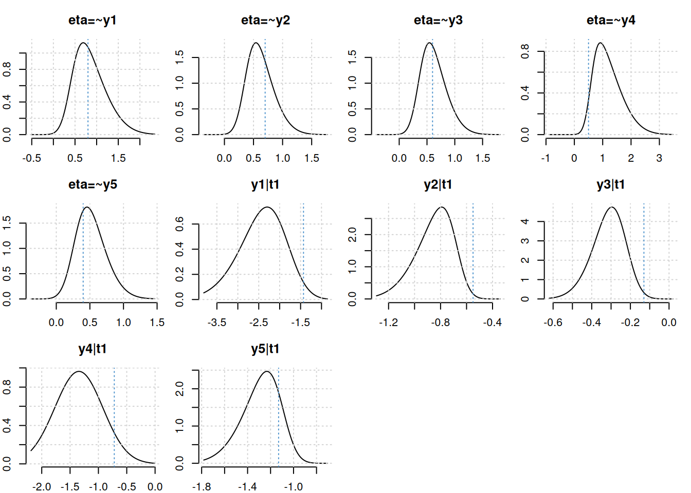
plot(fit, truth = truval)