library(INLAvaan)
mod <- "
    # Latent variable definitions
    ind60 =~ x1 + x2 + x3
    dem60 =~ y1 + y2 + y3 + y4
    dem65 =~ y5 + y6 + y7 + y8

    # Latent regressions
    dem60 ~ ind60
    dem65 ~ ind60 + dem60

    # Residual correlations
    y1 ~~ y5
    y2 ~~ y4 + y6
    y3 ~~ y7
    y4 ~~ y8
    y6 ~~ y8
  "
dat <- lavaan::PoliticalDemocracy

# Simulate missingness (MCAR)
set.seed(221)
mis <- matrix(rbinom(prod(dim(dat)), 1, 0.99), nrow(dat), ncol(dat))
datmiss <- dat * mis
datmiss[datmiss == 0] <- NAINLAvaan handles missing data in one of two ways: listwise deletion (default, i.e. uses all complete cases) or Full Information Maximum Likelihood (FIML; missing = "ML").
Simulate Data
Listwise Deletion
fit1 <- asem(mod, datmiss, meanstructure = TRUE)
#> ℹ Mode finding and Hessian computation.
#> ✔ Posterior mode and Hessian. [254ms]
#>
#> ℹ Performing VB correction.
#> ✔ VB correction; mean |δ| = 0.223σ. [503ms]
#>
#> ⠙ Fitting 0/42 skew-normal marginals.
#> ⠹ Fitting 23/42 skew-normal marginals.
#> ✔ Fit 42/42 skew-normal marginals. [2.3s]
#>
#> ℹ Adjusting copula correlations (NORTA).
#> ✔ Adjust copula correlations (NORTA). [285ms]
#>
#> ⠙ Posterior sampling and summarising.
#> ✔ Summarise 1000 posterior draws. [1.4s]
#>
#> ℹ Fit measures: PPP, DIC, LOO, WAIC.
fit1@Data@nobs[[1]] == nrow(datmiss[complete.cases(datmiss), ])
#> [1] TRUE
print(fit1)
#> INLAvaan 0.2.5.9004 ended normally after 71 iterations
#>
#>   Estimator                                      BAYES
#>   Optimization method                           NLMINB
#>   Number of model parameters                        42
#>
#>                                                   Used       Total
#>   Number of observations                            35          75
#>
#> Model Test (User Model):
#>
#>    Marginal log-likelihood                    -818.479
#>    PPP (Chi-square)                              0.506
coef(fit1)
#>    ind60=~x2    ind60=~x3    dem60=~y2    dem60=~y3    dem60=~y4    dem65=~y6
#>        1.808        1.750        0.943        0.805        1.472        1.061
#>    dem65=~y7    dem65=~y8  dem60~ind60  dem65~ind60  dem65~dem60       y1~~y5
#>        0.721        1.354        0.913        0.567        1.080        0.469
#>       y2~~y4       y2~~y6       y3~~y7       y4~~y8       y6~~y8       x1~~x1
#>        1.844        3.596        0.607       -0.669        1.283        0.071
#>       x2~~x2       x3~~x3       y1~~y1       y2~~y2       y3~~y3       y4~~y4
#>        0.144        0.424        1.698        7.790        4.086        2.786
#>       y5~~y5       y6~~y6       y7~~y7       y8~~y8 ind60~~ind60 dem60~~dem60
#>        1.537        6.752        2.038        3.983        0.506        1.439
#> dem65~~dem65         x1~1         x2~1         x3~1         y1~1         y2~1
#>        0.139        5.424        5.534        4.107        7.250        6.635
#>         y3~1         y4~1         y5~1         y6~1         y7~1         y8~1
#>        8.307        6.834        6.639        5.224        8.267        6.157
Full Information Maximum Likelihood (FIML)
fit2 <- asem(mod, datmiss, missing = "ML", meanstructure = TRUE)
#> ℹ Mode finding and Hessian computation.
#> ✔ Posterior mode and Hessian. [467ms]
#>
#> ℹ Performing VB correction.
#> ✔ VB correction; mean |δ| = 0.194σ. [596ms]
#>
#> ⠙ Fitting 0/42 skew-normal marginals.
#> ⠹ Fitting 19/42 skew-normal marginals.
#> ✔ Fit 42/42 skew-normal marginals. [4s]
#>
#> Warning in sqrt(Vx): NaNs produced
#> Warning in sqrt(Vx): NaNs produced
#> Warning in sqrt(Vx): NaNs produced
#> Warning in sqrt(Vx): NaNs produced
#> Warning in sqrt(Vx): NaNs produced
#> Warning in sqrt(Vx): NaNs produced
#> Warning in sqrt(Vx): NaNs produced
#> Warning in sqrt(Vx): NaNs produced
#> Warning in sqrt(Vx): NaNs produced
#> Warning in sqrt(Vx): NaNs produced
#> Warning in sqrt(Vx): NaNs produced
#> Warning in sqrt(Vx): NaNs produced
#> Warning in sqrt(Vx): NaNs produced
#> Warning in sqrt(Vx): NaNs produced
#> Warning in sqrt(Vx): NaNs produced
#> Warning in sqrt(Vx): NaNs produced
#> Warning in sqrt(Vx): NaNs produced
#> Warning in sqrt(Vx): NaNs produced
#> Warning in sqrt(Vx): NaNs produced
#> Warning in sqrt(Vx): NaNs produced
#> Warning in sqrt(Vx): NaNs produced
#> Warning in sqrt(Vx): NaNs produced
#> Warning in sqrt(Vx): NaNs produced
#> Warning in sqrt(Vx): NaNs produced
#> Warning in sqrt(Vx): NaNs produced
#> Warning in sqrt(Vx): NaNs produced
#> Warning in sqrt(Vx): NaNs produced
#> Warning in sqrt(Vx): NaNs produced
#> ℹ Adjusting copula correlations (NORTA).
#> ✔ Adjust copula correlations (NORTA). [298ms]
#>
#> ⠙ Posterior sampling and summarising.
#> ⠹ Computing WAIC.
#> ✔ Summarise 1000 posterior draws. [1.9s]
#>
#> ℹ Fit measures: PPP, DIC, LOO, WAIC.
print(fit2)
#> INLAvaan 0.2.5.9004 ended normally after 93 iterations
#>
#>   Estimator                                      BAYES
#>   Optimization method                           NLMINB
#>   Number of model parameters                        42
#>
#>   Number of observations                            75
#>   Number of missing patterns                        19
#>
#> Model Test (User Model):
#>
#>    Marginal log-likelihood                   -1415.513
#>    PPP (Chi-square)                              1.000
coef(fit2)
#>    ind60=~x2    ind60=~x3    dem60=~y2    dem60=~y3    dem60=~y4    dem65=~y6
#>        2.703        2.413        1.375        1.236        1.438        1.839
#>    dem65=~y7    dem65=~y8  dem60~ind60  dem65~ind60  dem65~dem60       y1~~y5
#>        1.567        1.963        3.014        1.500        1.094        3.908
#>       y2~~y4       y2~~y6       y3~~y7       y4~~y8       y6~~y8       x1~~x1
#>        6.535       11.466        3.516        4.883        7.183        0.207
#>       x2~~x2       x3~~x3       y1~~y1       y2~~y2       y3~~y3       y4~~y4
#>        1.016        1.008        5.546       14.907        6.945        6.979
#>       y5~~y5       y6~~y6       y7~~y7       y8~~y8 ind60~~ind60 dem60~~dem60
#>        4.439       12.553        4.898        8.195        0.980       11.150
#> dem65~~dem65         x1~1         x2~1         x3~1         y1~1         y2~1
#>       11.336        5.060        4.791        3.557        5.462        5.780
#>         y3~1         y4~1         y5~1         y6~1         y7~1         y8~1
#>        7.155        5.250        5.354        4.104        6.853        4.423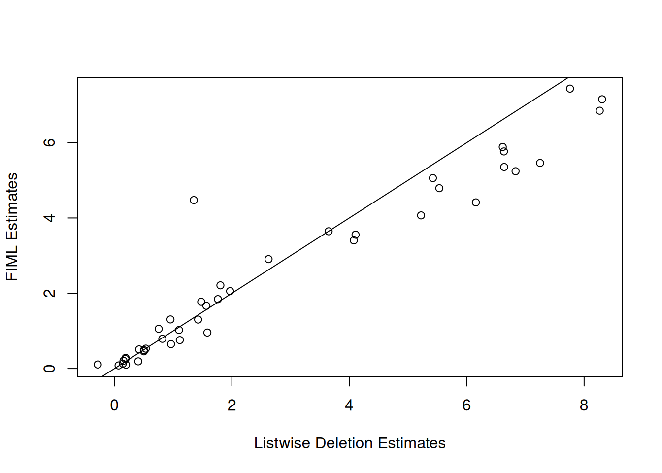
Model criteria under FIML
loo() and waic() work directly on a FIML fit. Each unit is scored on the entries it actually has – the observed-data predictive , with the full row deleted from the conditioning set – so a case with more missing entries contributes a smaller log-likelihood term and a smaller score, self-weighting in the expected log predictive density. The missing-at-random assumption that justifies FIML estimation also justifies this predictive score.
loo(fit2)
#> Taylor leave-one-subject-out cross-validation (INLAvaan)
#> Computed from 75 subjects (second-order Taylor approximation)
#>
#>          Estimate   SE
#> elpd_loo  -1285.5 36.5
#> p_loo        37.1  3.1
#> looic      2571.0 73.0
Comparing two FIML fits with compare(..., loo = TRUE) is valid only when they share the same observed entries – the same data and the same missingness pattern – since each unit is scored on the entries it has. See the cross-validation article for the Taylor case-deletion method itself.
Two-level FIML fits are also supported: they are scored per cluster (leave-one-cluster-out), each cluster contributing its observed-data marginal likelihood. The per-row deletion diagnostic (type = "loso") is not available under missing data.